Insights / Gulf · RAM
The Capacity That Survives a Failure Is Chosen at Concept Stage
What Habshan, Barzan and Pearl GTL show about train count, design margin and spares, and how to price them before FEED.
Habshan, onshore Abu Dhabi, is one of the largest gas processing sites in the region: five plants, 14 processing trains, 6.1 bscfd. ADNOC Gas reported two security-related incidents at the site on 3 and 8 April. Shortly afterwards 60% of processing capacity was back in service, and the company kept meeting domestic demand through its broader network. By August 85% was restored, ahead of the year-end target, with full capacity expected in the second quarter of 2027.
Two other Gulf plants show the other side. In Qatar, an explosion at the Barzan gas plant in June removed 35% of the country's 4 bcfd domestic gas supply, according to Wood Mackenzie. At Pearl GTL, one of the two trains was damaged in March, and Shell reported a partial restart in October, six months later.
I am not analysing the incidents or the security response, only what each plant's architecture did with the damage. Three numbers shaped the commercial outcome: the share of capacity that survived, how fast the rest came back, and whether the network could cover the gap. Repair crews influence the second. All three are bounded much earlier, at concept stage: how many trains, how large, how far apart, which utilities they share, and what other routes the gas has. That is the territory of RAM, and in the Gulf in 2026 it is not a theoretical exercise.
In short
- Design margin is redundancy nobody counts. With a 10% margin a "50%" train carries 55% of plateau, so margin and train count are one decision.
- Beyond N+1, more capacity buys almost nothing. Every layout that can lose a train and still carry plateau stops at the same 96.6% ceiling, set by single items such as the export pump.
- A Pre-FEED RAM study produces a boundary, not a winner. Four different layouts win across gas price and CAPEX accuracy; the deliverable is where each one wins.
- The bad year is set by spares policy. Spares moved the P10 year by 29 points; train configuration moved it by 4.
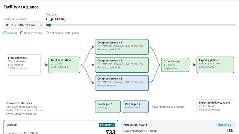
You can test every number below in the interactive RAM demonstrator. It opens in Base view: three findings, four inputs, the facility schematic and the decision map, readable in two minutes. Advanced view adds every input, the FEL 1 screen, five more robustness checks, the FEED Monte Carlo simulation and the formulas.
What RAM actually measures
Reliability is how long equipment runs before it fails (MTBF). Availability is the share of time a system can do its job: MTBF / (MTBF + MTTR). Maintainability is how quickly it comes back (MTTR), which depends as much on access, spares and repair crews as on the equipment itself.
For an investment decision the number that counts is production efficiency: delivered volume divided by what the reservoir and the market would have taken. RAM converts equipment behaviour into that figure, and the figure into deferred revenue. In RPV terms (Economic Potential x Delivery Certainty), it is the part of Delivery Certainty that has to survive after start-up.
The production assurance standard was reissued as ISO 20815:2026 in June. It frames production assurance as a process that runs through every life-cycle phase of an asset. Most projects still treat it as a FEED report.
Design margin: the redundancy nobody counts
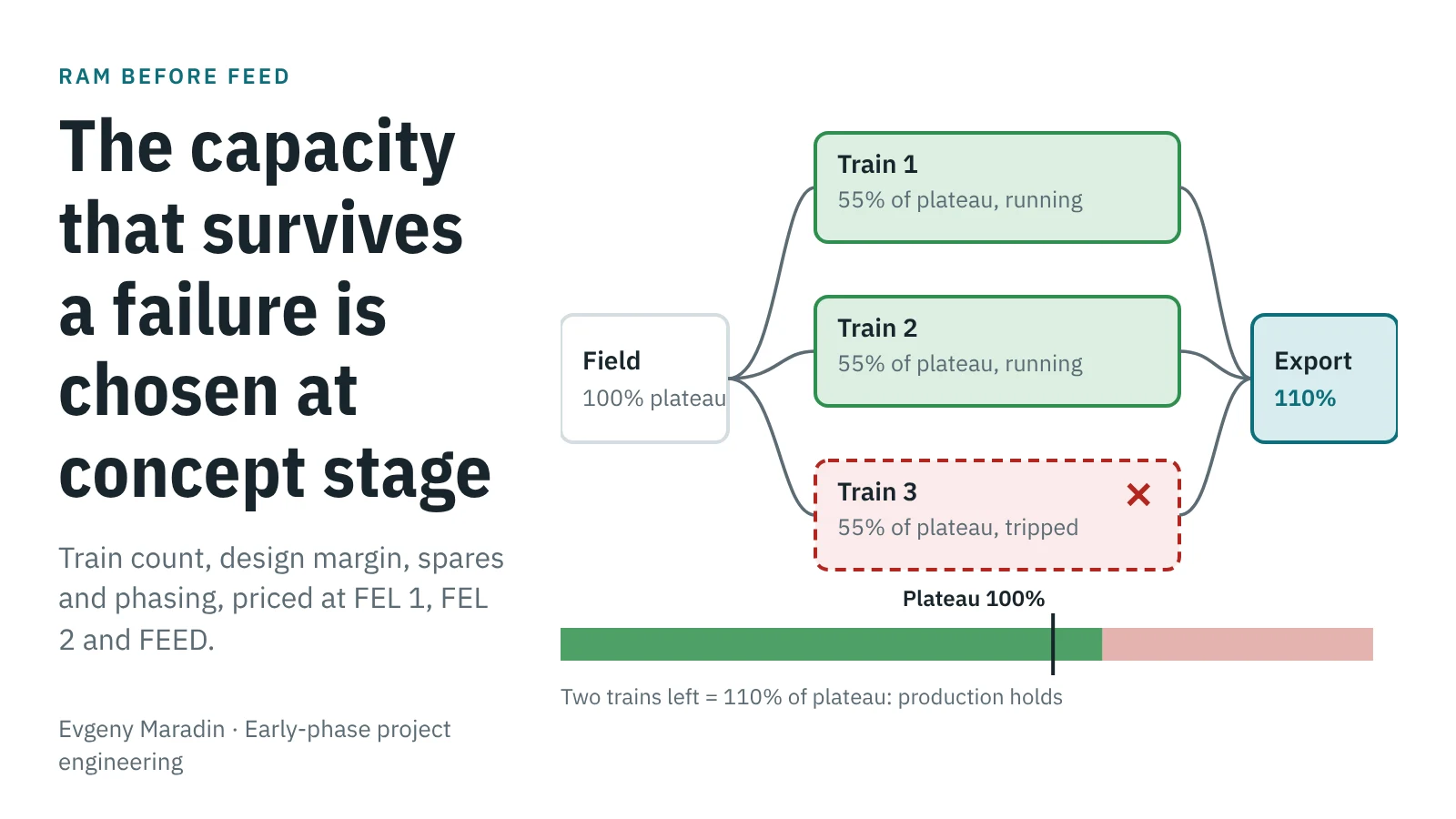
Every plant is built above its plateau rate. The margin sits in the design basis and is usually missing from the RAM model. In a multi-train plant that is a mistake, because the margin is partial redundancy.
No API, ISO or NORSOK standard fixes one plant-level margin. NORSOK P-100 makes design margin and turndown the project owner's call, and ISO 20815 with ISO 15663 expect that call to be justified by production assurance and lifecycle cost. Equipment standards give anchors: NORSOK P-002 sets at least 10% over design rates for scrubbers, and API 617 sizes compressor drivers 10% above maximum absorbed power. Licensors commonly add 10% on flow, and engineers from Solar Turbines and Saudi Aramco have shown how such margins stack into oversized compressors.
The standards are clear on redundancy and silent on configuration. NORSOK P-100 puts gas compression in sparing class A, where a failure stops or cuts production for more than two hours. For some class A services, such as export pumps, it requires a spare unit or spare capacity; for compression it leaves the sparing to the project. Whether that is a second 100% train, a third 50% train or two 60% trains is the trade-off a RAM study exists to make.
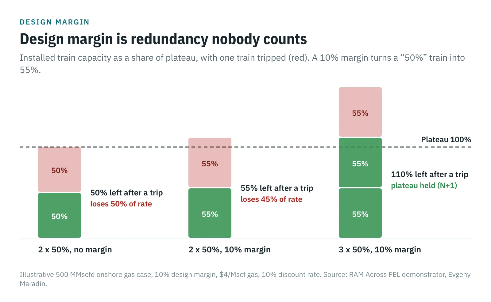
With a 10% margin, a single trip of a "50%" train costs 45% of the rate, not 50%. For a single train the margin buys nothing for availability; it adds catch-up capacity and raises the turndown floor. In the example below, moving the margin from 0% to 20% changes the lowest-cost layout from 3 x 50% to 2 x 60%. Margin and train count should be decided together.
The result most concept teams get wrong
To make this concrete I built the demonstrator around one illustrative onshore case: 500 MMscfd plateau, 10% design margin, a 20-year gas and condensate profile, and eight train layouts from 1 x 100% to 4 x 25%, including 2 x 100% and 4 x 33% with installed capacity well above plateau. The inputs are round screening values, not vendor data.
With no margin and no restart losses, splitting a 1 x 100% train into 2 x 50% gives exactly the same plateau production efficiency: 93.8% in both cases, because every lost train still takes half the plant with it. With the 10% margin and a 12-hour restart after every full-plant stop, the two trains reach 93.6% against 92.6%. The gain comes from the margin and from fewer full stops: about 4 a year instead of 9. It costs about $60M more compression CAPEX.
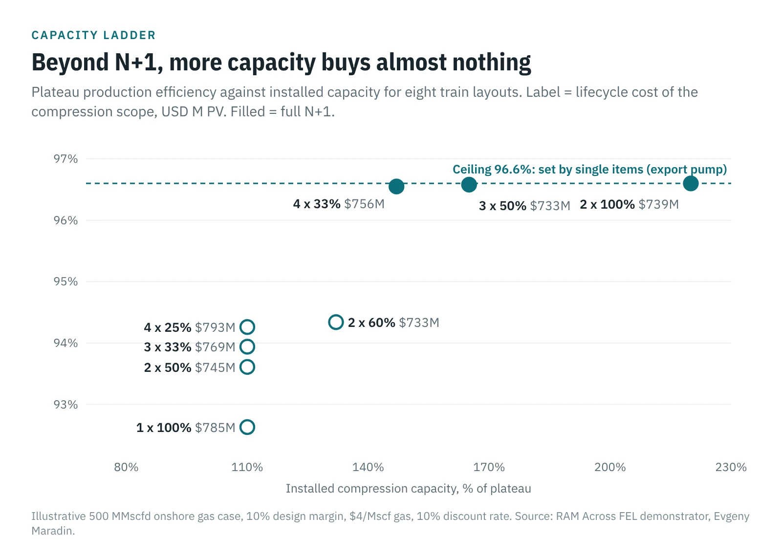
Plateau availability is bought with spare capacity, up to full N+1. 3 x 50%, with 165% installed capacity, reaches 96.6%. At $6,100 of revenue per MMscf, one point of plateau efficiency is worth about $11M a year.
Beyond N+1, more capacity buys almost nothing. 2 x 100% (220% installed) and 4 x 33% (147% installed) reach the same 96.6% ceiling. They cost $6M and $23M more than 3 x 50% over field life, and both are screened out at FEL 1. Adding or enlarging trains past N+1 is a decision about resilience to major events, catch-up or future tie-ins, and should be argued on those grounds.
Two trains also earn money in decline. Once demand falls below one train's capacity, the second becomes a spare. The turndown floor of 2 x 50% is reached in year 16 of this profile, against year 10 for a single train.
FEL 1: screen the architecture, not the number
At Concept there is no equipment list and no vendor. Train availability is a benchmark range (93% to 98% in the example) and CAPEX is a Class 5 estimate (-30% / +50%). The absolute ranges of all eight layouts overlap, and teams often conclude that nothing can be decided yet.
That conclusion is wrong. All options are estimated on the same benchmark set and the same cost basis, so their errors move together. Compared corner by corner (same availability case, same CAPEX accuracy), four layouts lose in every combination: 3 x 33% and 4 x 25% lose to 2 x 60%, and 2 x 100% and 4 x 33% lose to 3 x 50%. Four go forward.
The other FEL 1 outputs are structural: installed capacity against plateau, where the whole-plant single points of failure sit, what share of capacity survives the loss of one train area, when decline crosses each option's turndown floor, and how many tie-ins each option needs into the host. What FEL 1 must not do is report production efficiency to a decimal place.
| Stage | Method | Typical precision | Decisions it supports |
|---|---|---|---|
| FEL 1 Concept | Benchmark ranges, structural screening, dominance test | Several points | Drop dominated layouts; flag single points of failure, area-loss exposure, turndown, tie-ins |
| FEL 2 Pre-FEED | Block model: MTBF, MTTR, redundancy, common cause, restarts, host downtime | One to two points | Train count, margin and phasing; value spares; give the economic case a production efficiency and its boundary |
| FEED | Hourly Monte Carlo: crews, repair scatter, spares logistics | P10 to P90 band | Size spares and crews; set plateau commitments against the P10 year |
FEL 2: the answer is a boundary, not a winner
Pre-FEED has enough definition for a block model: MTBF and MTTR per block, common-cause failures, planned maintenance, host plant shutdowns and restarts. At base inputs the four carried layouts compare as follows.
| Layout | Lifecycle cost | Plateau efficiency | Installed | CAPEX | PV OPEX | PV deferment |
|---|---|---|---|---|---|---|
| 3 x 50% | $733M | 96.6% | 165% | $377M | $107M | $249M |
| 2 x 60% | $733M | 94.3% | 132% | $281M | $80M | $373M |
| 2 x 50% | $745M | 93.6% | 110% | $252M | $71M | $422M |
| 1 x 100% | $785M | 92.6% | 110% | $191M | $54M | $541M |
Against the single train, 3 x 50% spends $186M more CAPEX and $53M more PV OPEX to avoid $292M of PV deferment.
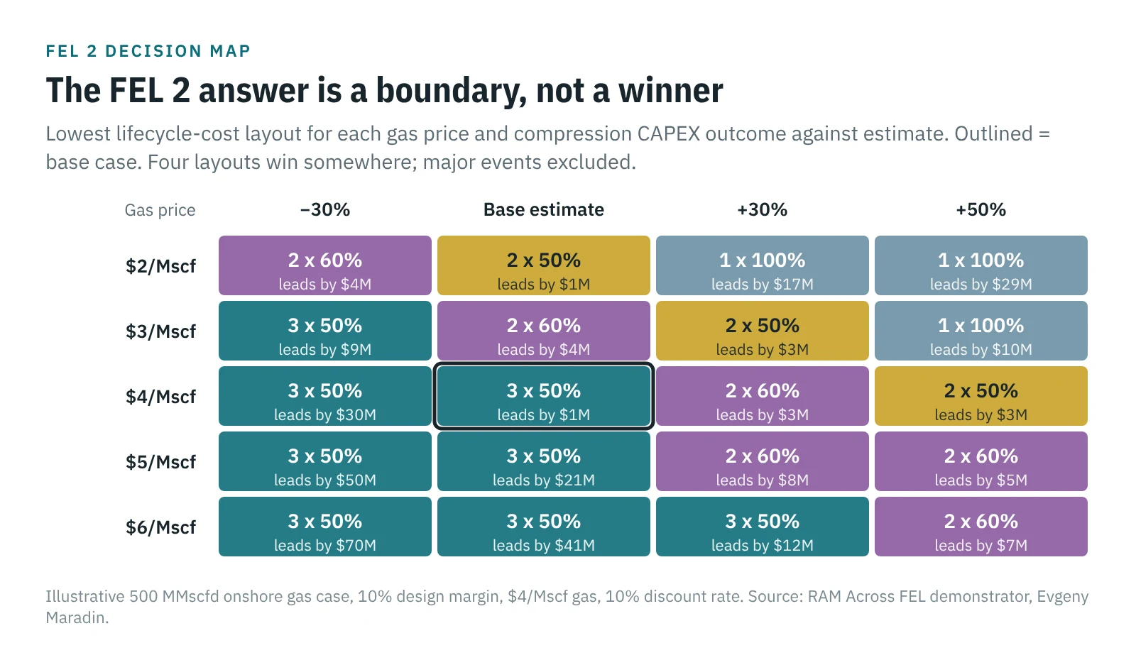
Then I stress-tested it. Rerun across gas price and CAPEX accuracy, the model produces a map with four different winners. At $4/Mscf and base CAPEX, 3 x 50% leads by $1M. With a 30% overrun on the compression estimate, 2 x 60% wins; with 50%, 2 x 50%. At $2 to $3/Mscf combined with an overrun, the single train wins. A three-year plateau, a train MTBF of 4,000 hours or a 20% design margin also move the answer to 2 x 60%.
So the FEL 2 deliverable is not "Option D". It is: two trains of 60% or three of 50%, a choice worth less than $5M at base inputs and settled by CAPEX accuracy; a single train only if gas is worth less than about $3/Mscf and the estimate grows. An investment board can test that sentence. It cannot test a single ranking.
Spares follow the same logic. For 3 x 50%, a second export pump at $25M avoids $70M of PV deferment and an N+1 generator at $30M avoids $42M. Both earn their place because every failure of a single item is also a full-plant stop and a restart.
Phasing: build capacity in steps, not redundancy
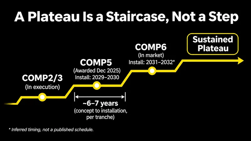
Trains have a second value that pure availability models miss: they can be built in stages. Phase 1 is sized for what the reservoir has proven, and later trains follow as appraisal and early production confirm the upside. If production comes in lower or later, the next train slips or is never built. CAPEX and OPEX then follow the field rather than the forecast made at FID.
In the example, a third 50% train that turns out not to be needed saves $126M of CAPEX, about $161M in PV once its OPEX is included. That is the value of keeping the decision open.
Later trains should be timed against the operator's portfolio, not only against this field. The question for train 3 is when the hub needs the capacity: this field's upside, a satellite waiting for a tie-in, or another project competing for the same capital. That turns a facility decision into a portfolio sequencing decision, which is where it belongs.
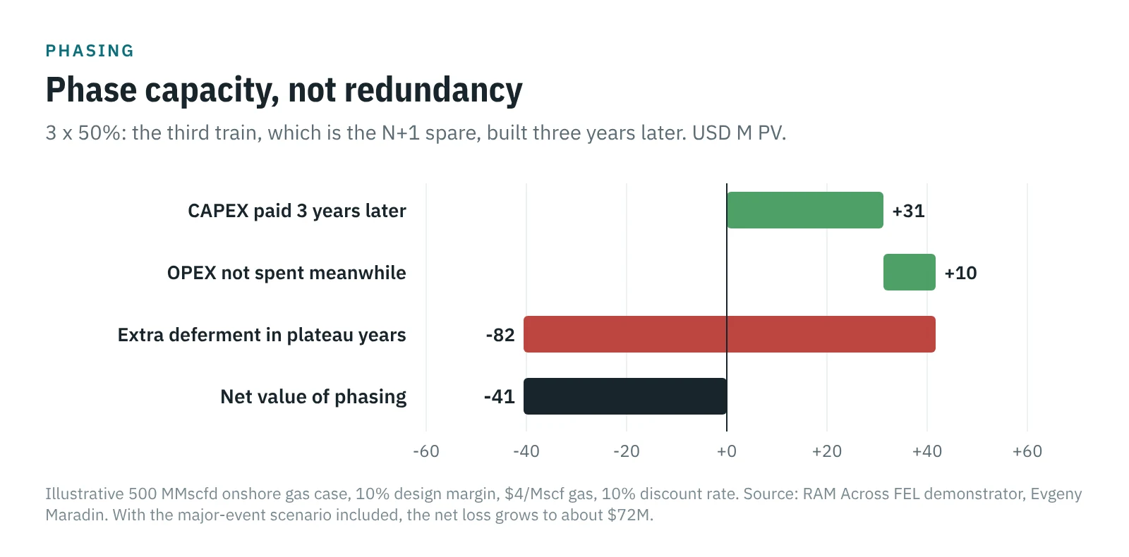
There is one trap: phase capacity, not redundancy. If the third train is the N+1 spare, deferring it by three years saves about $42M in PV ($31M from paying the CAPEX later, $10M of avoided OPEX) and costs about $82M of extra deferment in exactly the plateau years, when availability is worth most. Net, minus $41M. With the major-event scenario included, the loss grows to about $72M. The rule for FEL: make phase 1 resilient at the proven rate, and phase the trains that add capacity for the upside.
In brownfield there is a precondition. Every later train is a tie-in into a live plant. Plot space, headers with isolation valves, utilities laid out for expansion and tie-in points that do not need a full shutdown are cheap at FEL and expensive afterwards.
Major events: RAM on a different clock
Random failures are measured in hours. Fire, explosion or external damage is measured in months, and it takes out an area rather than one machine. Standard availability models leave this out, and it is exactly the case the Gulf has been living through this year.
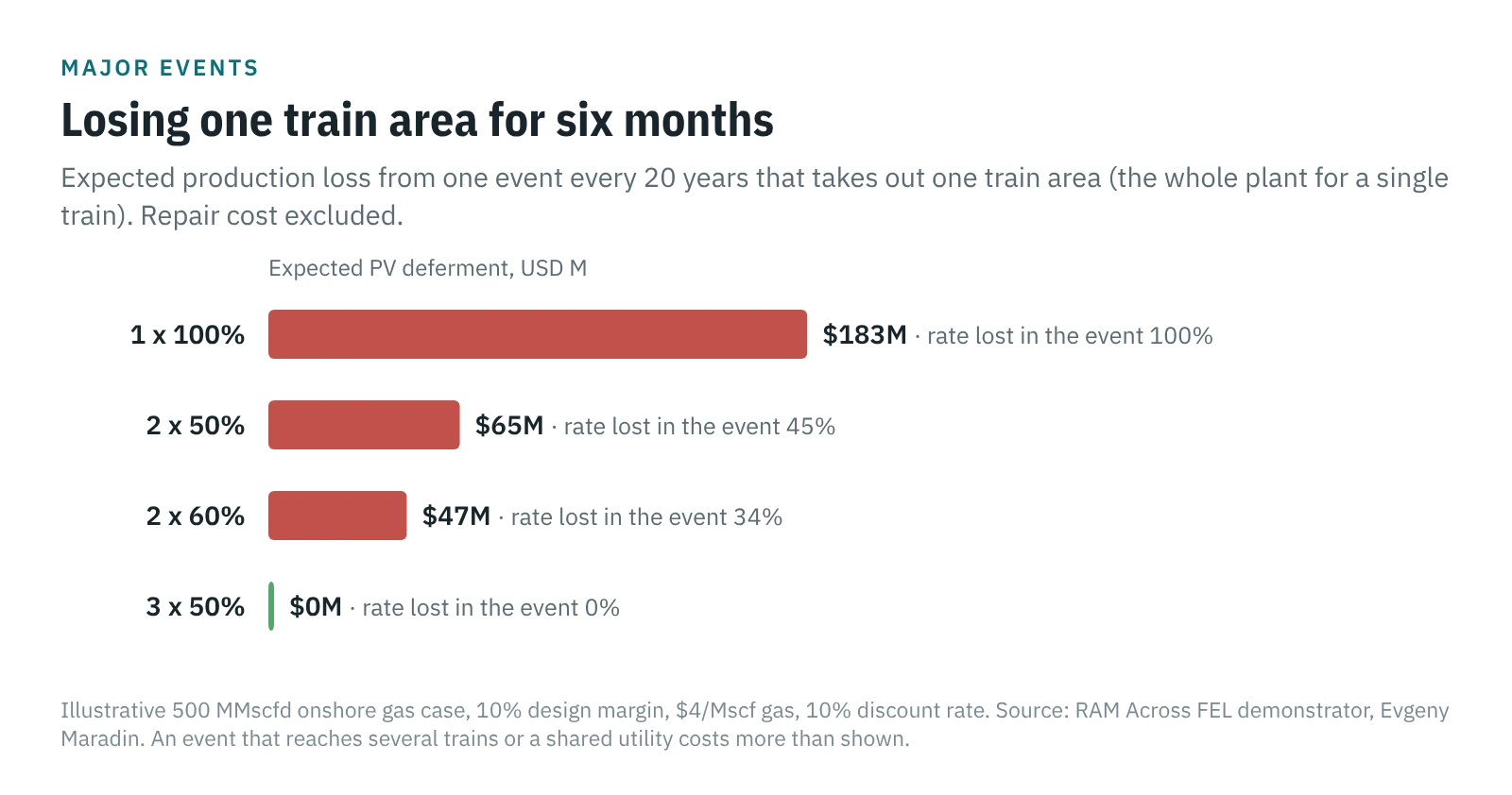
The demonstrator adds one scenario: once every 20 years, one train area is lost for six months. The expected PV deferment is $183M for 1 x 100%, $65M for 2 x 50%, $47M for 2 x 60%, and zero for 3 x 50%, because the remaining trains still carry plateau. With this scenario included, 3 x 50% wins at $3/Mscf and above, except where the compression estimate overruns by 30% at $3 or by 50% at $4.
Two cautions. The frequency is an input for the operator's risk and security teams, not for the concept engineer to guess. And the scenario assumes an event stays inside one train area. When one event can reach several trains or a shared utility, train count alone does not buy resilience. Spacing, segregation of utilities and alternative routes for the gas do, and each of them is a plot-plan decision made at concept stage.
What a deferred molecule is worth
The input that moves the result most is commercial, not mechanical. The model values deferred gas as lost in the year it happens. If the reservoir gives it back later, the credit is small: at a 10% discount rate, a molecule recovered in year 21 is worth about 13 cents on the dollar today.
Where plant gas feeds domestic power through a Gulf summer, a missed molecule is usually replaced by something more expensive rather than delivered later. Barzan's share of Qatar's domestic supply shows how concentrated that exposure can be. Where gas is sold under take-or-pay terms or into an LNG programme, the contract sets the cost. Either way, this is a number the commercial team owns, and it belongs in the RAM model at FEL 2, not in a footnote.
Brownfield: the host plant is inside your availability model
After gas price, the largest drivers of deferment for 3 x 50% are host plant shutdown days and the single export pump, then restart time. Compressor reliability sits near the bottom. Raising host shutdowns from 5 to 7.5 days a year adds about $49M of PV deferment.
This is constraint migration inside the facility. Once the trains are N+1, the binding constraint moves to whatever is still single: the export pump, the tie-in to the existing plant, the host's turnaround calendar. Those are interface questions answered by operations, not by vendors, and they need to be on the table at FEL 2.
FEED: the average is not the year you live through
At FEED the block model is replaced by an hour-by-hour Monte Carlo simulation with repair crews, scatter in repair time, spares logistics and restarts. With spares on site, the simulated mean for 3 x 50% is 96.5% against 96.6% from the FEL 2 model, with a P10 year of 94.3%. That agreement is the check that the model is built correctly.
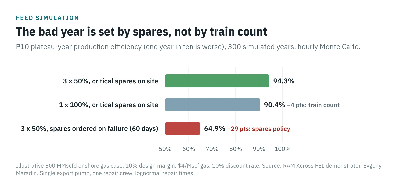
Then switch critical spares to ordered on failure with a 60-day lead time. The P50 year for 3 x 50% falls to 85.5% and the P10 year to 64.9%. A single 100% train with spares on site has a P10 year of 90.4%. Spares policy moved the bad year by 29 points; train configuration moved it by 4. The driver is the single export pump with no part on site. After a major event the same logic scales up: recovery curves depend on long-lead equipment, contractor capacity and repair access as much as on the damage itself.
Try it yourself
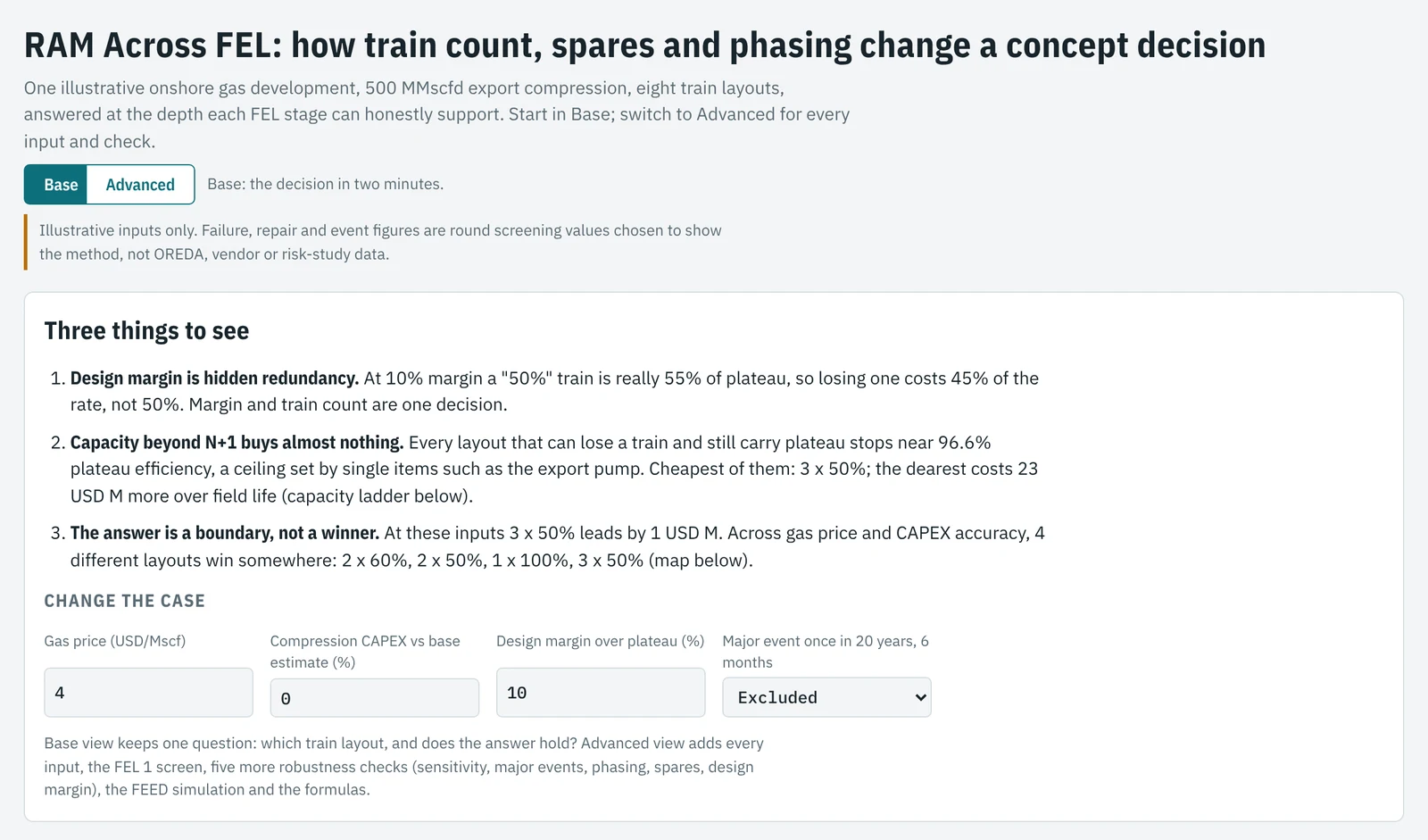
The RAM demonstrator runs in the browser, with no install. Base view answers one question, which train layout and does the answer hold, with four inputs: gas price, CAPEX against estimate, design margin and the major-event scenario. Advanced view is for engineers who want the method: every reliability and cost input, the FEL 1 dominance screen, sensitivity, major events, phasing, spares and margin checks, the FEED simulation and the formulas. All article figures come from its default inputs.
What RAM is not
RAM is a production assurance tool. It is not asset integrity management, process safety or security risk assessment. It does not tell you how likely an event is or how to prevent it. It tells you what the event costs in production, given the architecture you chose, so that the people who set protection budgets and the people who choose train counts work from the same number.
Six questions to ask before FEED
- What production efficiency does the economic case assume, and who owns that number?
- What design margin over plateau is assumed, and has it been counted as partial redundancy?
- What is a deferred molecule worth under the sales arrangement, and who signed off that value?
- Which single item stops the whole plant, how often, and how long is a realistic outage including parts, access and restart?
- What capacity survives the loss of one train area or one shared utility, and for how many months?
- Are host plant shutdowns and tie-in windows inside the availability model?
Calculation note
- Revenue per MMscf: 1,000 Mscf x $4.0 + 30 bbl condensate x $70 = $6,100.
- One point of plateau efficiency: 500 MMscfd x 365 x 1% = 1,825 MMscf/yr, about $11M/yr.
- Installed train size = nominal size x 1.10 (design margin). Compression CAPEX, six-tenths rule: train cost = $180M x (installed size)^0.6. 1 x 100% = $191M; 2 x 50% = $251M; 3 x 50% = $377M; 2 x 100% = $381M.
- Full-plant stops per year, 1 x 100%: compressor trips 8,760 / 2,000 h = 4.4; inlet separation 1.0; export pump 1.5; pipeline 0.2; host turnaround 1; train maintenance 1; total about 9.0. Multi-train layouts: about 4.0, because a single compressor trip no longer stops the plant.
- 3 x 50% vs 1 x 100% at base inputs: CAPEX +$186M, PV OPEX +$53M, PV deferment -$292M, net lifecycle saving about $52M (10% discount rate, 6-year plateau, 12%/yr decline, 20-year life, 12-hour restart, major events excluded).
- Major-event scenario, 1 x 100% at plateau: 1/20 per year x 0.5 year = 2.5% expected outage; 2.5% x 500 MMscfd x 365 x $6,100 = about $28M/yr. Over the profile at 10%: $183M PV.
- Phasing, 3 x 50%, third train deferred 3 years: CAPEX $126M x (1 - 1/1.1^3) = $31.3M; avoided OPEX $10.4M PV; together $41.7M. Extra deferment in years 1-3 = $82.2M PV; net -$40.6M, about -$41M. Never built: $126M CAPEX + $36M PV OPEX = $161M (rounded).
- Recovery credit: discount factor for year 21 at 10% = 1 / 1.1^21 = 0.135.
- Habshan: 15% of 6.1 bscfd = about 0.9 bscfd still to restore after August. My calculation from the reported figures.
- Design margin references: NORSOK P-100 cl. 4.2.4 (margin and turndown set by the project owner), cl. 5.3.2 (20% scrubber margin for control fluctuations), sparing classes A/B/C (cl. 3.1), gas compression class A (cl. 9.2.3); NORSOK P-002 (at least 10% on scrubber design rates); API 617 (driver at least 110% of maximum absorbed power); API 675 (metering pump rated capacity at least 110% of maximum specified).
- All reliability and event inputs are illustrative screening values, not OREDA, vendor or risk-study data.
Working on a concept, Pre-FEED or a tender pack? A short call is often enough to see where the gaps are.